Basic probability theory, MT3001 module 1 / 15
Introduction
Probability theory is the study of random phenomena. It is used in many fields, such as statistics, machine learning, and finance. It is also used in everyday life, for example when playing games of chance, or when estimating the risk of an event. The most classic example is the coin toss, closely followed by the dice roll.
When we toss a coin, the result is either heads or tails. In the case of an ideal coin, the "random trail" of tossing the coin has an equal probability for both outcomes. Similarly, for a die roll of a fair dice, we know that the probability for each outcome is 1/6. In the study of probability we dive deep into the mathematics of these random phenomena, how to model them, and how to calculate the probability of different events. To do this in precise terms, we define words and concepts as tools for discussing and communicating about the subject.
This is the first of what I expect to be a 15 part series of my lecture & study notes from my university course in probability theory MT3001 at Stockholm University. References to definitions and theorems will use their numeration in the course literature, even if I may rephrase them myself. The book I've had as a companion through this course is a Swedish book called Stokastik by Sven Erick Alm and Tom Britton; ISBN:978-91-47-05351-3. This first module concerns basic concepts and definitions, needed for the rest of the course.
The language of Probability theory
An experiment is a process that produces a randomized result. If our experiment is throwing a die, we then have the following: The result of throwing the die is called an outcome, the set of all possible outcomes is called the sample space and a subset of the sample space is called an event. We will use the following notation:
- outcome is the result of an experiment, denoted with a small letter, ex. \(u_1\), \(u_2\), \(u_3\), ...
- event is the subset of the sample space, denoted with a capital letter, ex. \(A\), \(B\), \(C\), ...
- sample space is the set of all possible outcomes of an experiment, denoted \(\Omega\).
Adding numbers to our dice example, we have the sample space \(\Omega = \{1,2,3,4,5,6\}\) containing all the possible events \(u_1=1, u_2=2, u_3=3, u_4=4, u_5=5\) and \(u_6=6\). And we could study some specific sub events like the chance of getting an even number, \(A=\{2,4,6\}\), or the chance of getting a prime number, \(B=\{2,3,5\}\). As it happens, the probability of both \(A\) and \(B\) is 50%.
Sample space
The sample space is the set of all possible outcomes of an experiment. It is denoted \(\Omega\). And there are two types of sample spaces, discrete and continuous. A discrete sample space is a finite or countably infinite set, and all other kind of sample spaces are called continuous.
The coin toss and the dice roll are both examples of discrete sample spaces. Studying a problem, like the temperature outside, would in reality require a continuous sample space. But in practice, we can often approximate a continuous sample space with a discrete one. For example, we could divide the temperature into 10 degree intervals, and then we would have a discrete sample space.
Remember that continuous sample spaces exist, and expect more information about them in later modules. For starters, we focus on discrete sample spaces.
Set Theory notation and operations
When talking about probabilities we will arm ourselves with the language of "set theory", it is a crucial tool for the study of probability. Feeling comfortable with the subject of set theory since before is useful, but not necessary. I will try to explain the concepts as we go along.
Even tough the events from the dice rolls are represented by numbers, it is important to note that they aren't numbers, but rather elements. This might become more clear if we alter our example to be a deck of cards. This deck of cards have four suits \(\Omega = \{\heartsuit, \spadesuit, \diamondsuit, \clubsuit \}\) and in our experiments we draw a card from the deck and look at the suit. It's here very obvious that we can't add or subtract the different events with each other. But we do have the operations of set theory at our disposal. For example, if \(A\) is the event of drawing a red card and \(B\) is the event of drawing spades \(\spadesuit\), we can use the following notation:
- \(A=\{\heartsuit, \diamondsuit\}\)
- \(B=\{\spadesuit\}\)
Set theory operations
- Union: \(A \cup B = \{\heartsuit, \diamondsuit, \spadesuit\}\), the union of \(A\) and \(B\).
- The empty set: \(\emptyset = \{\}\), the empty set. A set with no elements.
- Intersection: \(A \cap B = \emptyset\), the intersection of \(A\) and \(B\).
- This means that \(A\) and \(B\) have no elements in common. And we say that \(A\) and \(B\) are disjoint.
- Complement: \(A^c = \{\spadesuit, \clubsuit\}\), the complement of \(A\).
- Difference: \(A \setminus B = \{\heartsuit, \diamondsuit\}\), the difference of \(A\) and \(B\). Equivalent to \(A \cap B^c\).
- The symbol \(\in\) denotes that an element is in a set. For example, \(u_1 \in \Omega\) means that the outcome \(u_1\) is in the sample space \(\Omega\). For our example: \(\heartsuit \in A\) means that the suit \(\heartsuit\) is in the event \(A\).
Venn diagram
A very useful visualization of set theory is the Venn diagram. Here is an example of a Venn diagram in the picture below:
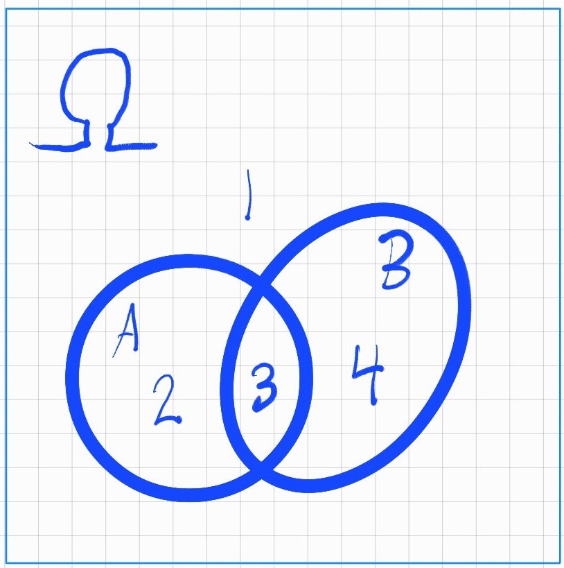
In the above illustration we have: \(\Omega = \{1,2,3,4\}\) and the two events \(A=\{2,3\}\) and \(B=\{3,4\}\). Notice how the two sets \(A\) and \(B\) share the element \(3\), and that all sets are subsets of the sample space \(\Omega\). The notation for the shared element \(3\) is \(A \cap B = \{3\}\).
Useful phrasing
The different set notations may seem a bit abstract at first, at least before you are comfortable with them. Something that might be useful to do is to read them with the context of probabilities in mind. Doing this, we can read some of the different set notations as follows:
- \(A^c\), "when \(A\) doesn't happen".
- \(A \cup B\), "when at least one of \(A\) or \(B\) happens".
- \(A \cap B\), "when both \(A\) and \(B\) happens".
- \(A \cap B^c\), "when \(A\) happens but \(B\) doesn't happen".
The Probability function
Functions map elements from one set to another. In probability theory, we are interested in mapping events to their corresponding probabilities. We do this using what we call a probability function. This function is usually denoted \(P\) and have some requirements that we will go through in the definition below.
This function take events as input and outputs the probability of that event. For the example of a die throw, if we have the event \(A=\{2,4,6\}\), then \(P(A)\) is the probability of getting an even number when throwing a fair six sided dice. In this case \(P(A)=\frac{1}{2}=P(\text{"even number from a dice throw"})\), you'll notice that variations of descriptions of the same event can be used interchangeably.
The Russian mathematician Andrey Kolmogorov (1903-1987) is considered the father of modern probability theory. He formulated the following three axioms for probability theory:
Definition 2.2, Kolmogorov's axioms
A real-valued function \(P\) defined on a sample space \(\Omega\) is called a >probability function if it satisfies the following three axioms:
- \(P(A) \geq 0\) for all events \(A\).
- \(P(\Omega) = 1\).
- If \(A_1, A_2, A_3, ...\) are disjoint events, then \(P(A_1 \cup A_2 \cup A_3 \cup ...) = P(A_1) + P(A_2) + P(A_3) + ...\). This is called the countable additivity axiom.
From these axioms it's implied that \(P(A) \in [0,1]\), which makes sense since things aren't less than impossible or more than certain. As a rule of thumb, when talking about probabilities, we move within the range of 0 and 1. This lets us formulate the following theorem:
Theorem 2.1, The Complement and Addition Theorem of probability
Let \(A\) and \(B\) be two events in a sample space \(\Omega\). Then the following statements are true: 1. \(P(A^c) = 1 - P(A)\) 2. \(P(\emptyset) = 0\) 3. \(P(A \cup B) = P(A) + P(B) - P(A \cap B)\)
Proof of Theorem 2.1
- \(P(A \cup A^c) = P(\Omega) = 1 = P(A) + P(A^c) \Rightarrow P(A^c) = 1 - P(A)\)
- This simply proves that the probability of \(A\) not happening is the same as the probability of \(A\) happening subtracted from 1.
- \(P(\emptyset) = P(\Omega^c) = 1 - P(\Omega) = 1 - 1 = 0\)
- Even though our formal proof required (1) to be proven, it's also very intuitive that the probability of the empty set is 0. Since the empty set is the set of all elements that are not in the sample space, and the probability of an event outside the sample space is 0.
- \(P(A \cup B) = P(A \cup (B \cap A^c)) = P(A) + P(B \cap A^c) = P(A) + P(B) - P(A \cap B)\)
- This can be understood visually by revisiting our Venn diagram. We see that the union of \(A\) and \(B\) has an overlapping element \(3\) shared between them. This means that purely adding the elements of \(A=\{2,3\}\) together with \(B=\{3,4\}\) would double count that shared element, like this \(\{2,3,3,4\}\), since we have two "copies" of the mutual elements we make sure to remove one "copy" bur removing \(P(A \cap B)=\{3\}\) and we get \(P(A \cup B)=\{2,3,4\}\). We may refer to this process as dealing with double counting, something that is very important to have in mind when dealing with sets.
Two interpretations of probability that are useful and often used are the frequentist and the subjectivist interpretations. The frequentist interpretation is that the probability of an event is the relative frequency of that event in the long run. The subjectivist interpretation is that the probability of an event is the degree of belief that the event will occur, this is very common in the field of statistics and gambling. For the purposes of study it's also useful to sometimes consider probabilities as areas and or masses, this is called the measure theoretic interpretation. Don't let that word scare you off, in our context it's just a fancy way of drawing a parallel between areas and probabilities. Think area under curves, and you'll be fine.